Lecture overview:

Total time: ~55 minutes
Prerequisites: L3 (ArrayList vs LinkedList), L14 (Debugging/Scientific Method), L20 (Networks), L31 (Threads), L32 (Async), L33 (Event Architecture)
Connects to: L35 (Safety and Reliability), L36 (Sustainability), GA1 (CookYourBooks performance)

Structure (~23 slides):

Arc 1: Big-O Notation (~10 min) — growth rates, recognizing complexity, constants
Arc 2: Measure, Don't Guess (~7 min) — profiling, flame graphs, performance dimensions
Arc 3: Architectural Decisions (~15 min) — memory hierarchy, latency budgets, architecture constraints
Arc 4: Performance Patterns (~10 min) — caching, batching, pooling, premature optimization
Arc 5: Garbage Collection (~8 min) — safety-performance trade-off, GC everywhere
Arc 6: Wrap-Up (~5 min) — comprehension check, sustainability, looking ahead

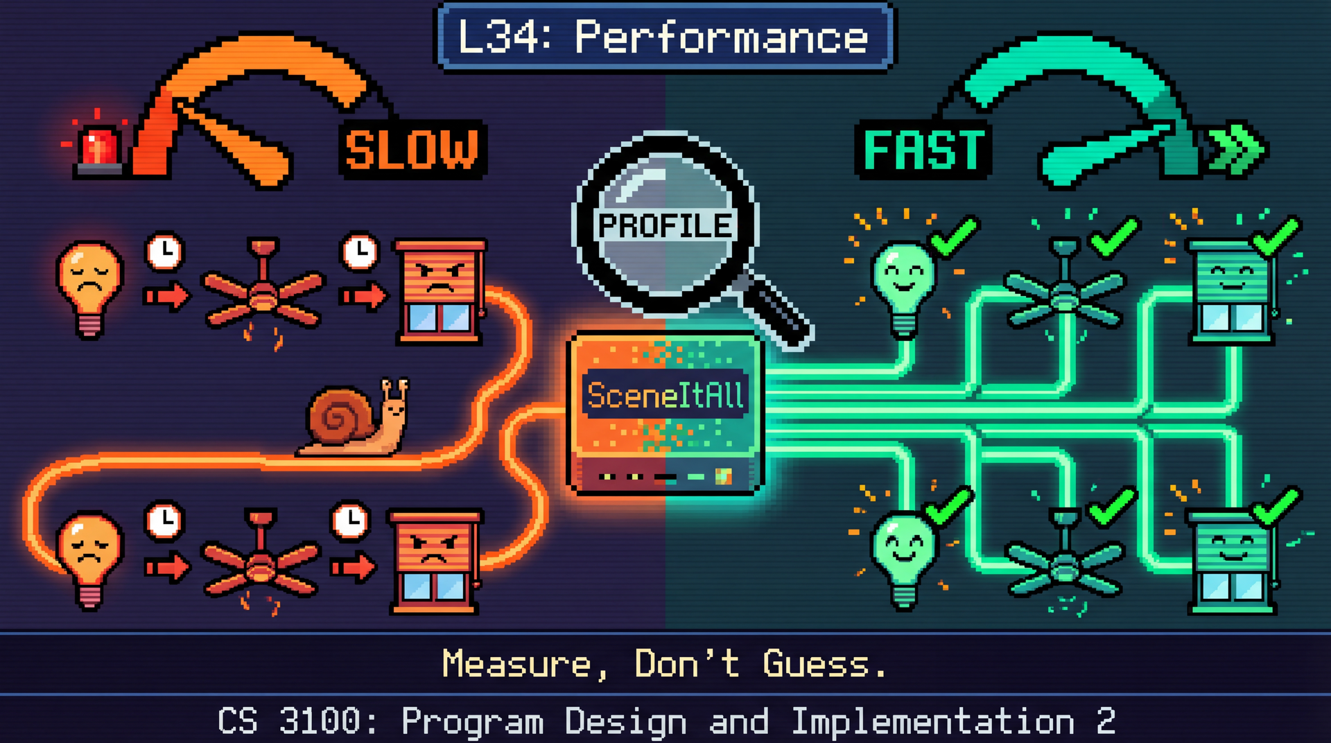
Running examples: SceneItAll (IoT hub performance) and Pawtograder (grading pipeline latency). These are systems students know and have experienced directly.

GA1 due Apr 9 — students are finishing CookYourBooks features. Performance is directly relevant: why their GUI freezes, why network calls are slow, why batching matters.

Transition: Let's start with the learning objectives...

CS 3100: Program Design and Implementation II

Lecture 34: Performance

Learning Objectives

After this lecture, you will be able to:

Reason about algorithmic growth using Big-O notation
Identify performance bottlenecks: measure, don't guess
Analyze the performance impact of architectural decisions
Apply common patterns to improve performance

Performance Touches Everything We've Learned — But Performance for Whom?

Lecture	Performance concept
L3 (Java Collections)	ArrayList vs LinkedList
L20 (Networks)	Network latency, caching
L31 (Concurrency I)	Thread overhead
L32 (Concurrency II)	I/O scaled-time table
L33 (Event Architecture)	Rate limiting

Today we bring those threads together. Core principle: measure, don't guess.

L14's scientific method applies here too — hypothesize, measure, iterate.

Big-O Describes How Code Scales, Not How Fast It Is

Notation	Name	SceneItAll example
O(1)	Constant	`HashMap` lookup by ID
O(log n)	Logarithmic	Binary search sorted devices
O(n)	Linear	Iterate all devices by name
O(n log n)	Linearithmic	Sort 1,000 devices
O(n²)	Quadratic	Compare every device pair

Recognize Complexity in Code Without Proofs

// O(1) — constant: one operation regardless of collection size
Device device = deviceMap.get(deviceId);

// O(n) — linear: one loop through the collection
for (Device d : devices) {
    if (d.getName().equals(name)) return d;
}

// O(n²) — quadratic: nested loops over the same collection
for (Device a : devices) {
    for (Device b : devices) {
        if (a != b && a.getRoom().equals(b.getRoom())) {
            // compare every pair — grows with n²
        }
    }
}

// O(n log n) — sorting
Collections.sort(devices, Comparator.comparing(Device::getBrightness));

The practical test: "If I double the input, how much slower?" O(n) = 2x. O(n²) = 4x.

Constants Don't Matter — Until They Do

// O(n) total: each ArrayList.get(i) is O(1)
for (int i = 0; i < arrayList.size(); i++) {
    process(arrayList.get(i));   // ~1 ns per element (cache-friendly)
}
// O(n²) total: each LinkedList.get(i) walks up to O(n) nodes
for (int i = 0; i < linkedList.size(); i++) {
    process(linkedList.get(i));  // pointer chasing; cache-unfriendly
}

Walking the whole list with an iterator is O(n) for both. But ArrayList is 10-100x faster due to cache locality.

"Big-O says they're the same. Your users disagree."

Big-O Matters When n Is Large — or When Each Operation Is Expensive

Big-O doesn't tell you about constant factors or GC pressure. "This is why we still need profiling."

You Cannot Trust Your Intuition About Where Time Is Spent

Code that looks slow may be irrelevant to overall runtime.

Code that looks fast may be called millions of times and dominate the profile.

"Is this method inherently expensive, or is it being called too many times?"

Inherently expensive → optimize the algorithm
Called too many times → cache or batch

Flame Graphs Show Where Time Goes

Simplified flame graph: computeOptimal() is a wide red bar (40% CPU, the bottleneck) while getById() is a tiny blue bar (2% CPU, negligible despite high call count)

Tools (know they exist, not details): JFR (Java Flight Recorder, built into JDK), flame graphs, heap dumps

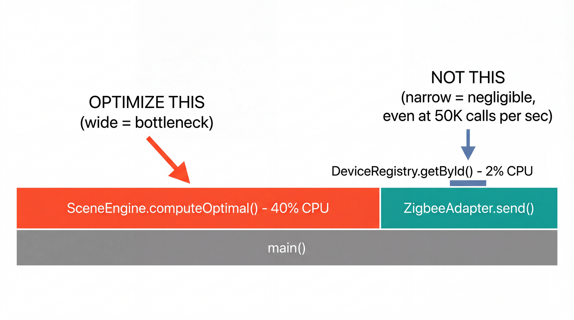
Flame graphs are the most useful profiling visualization. The width of each box represents the proportion of CPU time spent in that method. Wider = more time = higher priority to optimize.

The SceneItAll example concretizes the measurement principle:

computeOptimal() is called infrequently but is computationally expensive — it dominates the profile
getById() is called 50,000 times per second but each call is O(1) HashMap lookup — negligible total

This primes Poll Question Q2 where students must apply this reasoning.

Tools for reference:

JFR (Java Flight Recorder): Built into the JDK, low overhead, production-safe
Flame graphs: Visual representation of where CPU time goes
Heap dumps: Snapshot of all live objects — use when you suspect a memory leak

Transition: Performance isn't just about CPU time...

Performance Has Several Dimensions That Trade Off

Metric	What it measures	Example
Latency	Time for a single operation	"How long until the user sees their grade?"
Throughput	Operations per unit time	"How many submissions per minute?"
Memory	Heap/stack consumption	"How much RAM for 1,000 devices?"
CPU	Processor time consumed	"CPU-bound or I/O-bound?" (recall L32)

Optimizing one can worsen another: caching reduces latency but increases memory.

Data Location Determines Performance

Architecture determines where data lives. Monolith = RAM (5 min). Microservices = network (5 years).

ArrayList Wins Because of Cache Lines, Not Algorithms

Recall L3: "Use ArrayList by default." Now we explain why.

Both are O(n) to iterate. ArrayList is 10-100x faster because of cache locality.

Latency Budgets: Where Does the Time Actually Go?

Optimizing the 5ms computation to 1ms saves 4ms — irrelevant. Batching Zigbee saves 100ms+ — significant.

Hub runs great on Pi 5 — but 80% of deployed hubs are Pi 3s. Optimizing for modern hardware excludes existing users.

You've Lived Inside This Latency Budget

Infrastructure dominates everything. It typically takes 2-3 minutes just to go from push to running tests. Optimizing test execution from 10s to 8s saves 2s — irrelevant compared to the infrastructure overhead.

Amazon found every 100ms of added latency cost them 1% of sales. L20 Fallacy 2: latency is not zero.

Students have experienced this latency every time they submit. The infrastructure overhead — queuing the workflow, finding an available runner, provisioning the environment — takes 2-3 minutes. That's where the time goes. The grader tarball caching by SHA connects to L20's caching discussion.

Brief reference: architectural decisions that set the performance ceiling:

Monolith vs microservices: method calls (ns) vs network calls (ms) — L19
Synchronous vs async: blocking threads vs event-driven I/O — L32
Thread-per-request vs pool: memory scales with connections vs bounded — L31
Serverless vs always-on: cold start latency vs idle resource cost — L21

GitHub monolith note: GitHub is a Ruby on Rails monolith serving 100M+ developers. As AI-generated traffic doubled request volume, they optimized within the monolith — aggressive caching, database read replicas, request-level performance budgets — rather than rewriting as microservices. Sometimes the right move is to optimize within your architecture rather than change it.

L18 callback: Architecture determines the ceiling. You can optimize code within an architecture, but you can't exceed its fundamental limits.

Transition: Now that we know where time goes, how do we fix it?

Caching: The Fastest Operation Is the One That Doesn't Happen

Before: compute every time

public SceneSettings getSettings(
    Scene scene, SensorData sensors) {
  // 50ms each time
  return settingsEngine
    .computeOptimal(scene, sensors);
}

After: cache by inputs — O(f(n)) → O(1)

private final Map<CacheKey, SceneSettings>
    cache = new ConcurrentHashMap<>();

public SceneSettings getSettings(
    Scene scene, SensorData sensors) {
  return cache.computeIfAbsent(
    new CacheKey(scene.getId(),
      sensors.hash()),
    k -> settingsEngine
      .computeOptimal(scene, sensors));
}

Cache when: same inputs, staleness acceptable. Don't cache: inputs always change, or staleness is unsafe (L33).

L20 + L33 callback: In L20 we discussed caching as a network optimization — Pawtograder caches grader tarballs by SHA hash. In L33 we formalized this: a cache is an eventually consistent copy of the source of truth. The cache invalidation problem ("when does the cache expire?") is the consistency question in disguise.

Teaching point: Caching is the single most effective optimization pattern. It turns an O(f(n)) computation into O(1) for cache hits — you skip the computation entirely. With a 95% hit rate, you've effectively turned an expensive operation into a near-constant-time one.

ConcurrentHashMap.computeIfAbsent is the idiomatic Java way to implement a cache — it's thread-safe and only computes the value if the key isn't present.

Transition: Caching avoids redundant work. What about unavoidable work that has a high fixed cost?

Batching: Amortize the Fixed Cost Across Many Items

Before: 15 calls × 200ms = 3 seconds

for (Device device : devices) {
    zigbee.sendCommand(device, command);
}

After: 1 batch call = 200ms

zigbee.sendBatch(devices, command);

Where	The problem	The fix
Database	N queries for N records (N+1 problem)	One query with JOIN
Network	N API calls	Batch endpoint
File I/O	Write one byte at a time	Buffered writer

Pooling: Reuse Expensive Resources

// Thread pool: reuse threads instead of creating new ones per task
ExecutorService pool = Executors.newFixedThreadPool(10);

You've already used this pattern — ExecutorService in L31 is a thread pool.

Resource	Pool type	Why it matters
Threads	Thread pool (L31)	Each thread costs 512KB-1MB of stack
DB connections	Connection pool	Opening a connection: ~10ms TCP + auth
HTTP connections	HTTP keep-alive	Reuse TCP connections across requests

Creating the resource once and reusing it is always faster than creating and destroying per use.

Premature Optimization Is the Root of All Evil

"Premature optimization is the root of all evil." — Donald Knuth

Every optimization increases coupling (L7): cached values must be invalidated, batched operations add complexity, pooled resources must be managed.

Caching, batching, and pooling all create objects on the heap. Who cleans them up?

Automatic Memory Management Trades Performance for Safety

C/C++ (manual)

Full control over when memory is freed.

But: use-after-free, double-free, memory leaks. Among the most dangerous bugs in software engineering.

Java/Python/JS (automatic)

Garbage collector decides when to free.

You cannot use-after-free in Java. Trade-off: GC may pause your application at inconvenient times.

Automatic memory management is overwhelmingly the right default — the bugs it prevents are far more costly than the performance it sacrifices.

This is a design decision at the language level. It reflects the same safety-vs-performance trade-off we've seen throughout the course. Java's garbage collector eliminates entire categories of bugs — use-after-free, double-free, dangling pointers — at the cost of occasional GC pauses.

High allocation rate = more GC pauses: Caching, batching, and pooling all create objects. Those objects eventually become garbage. A high allocation rate means the GC runs more frequently, causing more pauses.

Pawtograder example: During deadline submission spikes, thousands of grading jobs allocate large data structures simultaneously. This creates heap pressure, triggers GC pauses, and can delay grade display — the same spike that stresses the system also stresses the garbage collector.

Transition: "But how dangerous are these manual memory bugs, really? Let me show you..."

Use-After-Free: How a PNG Can Root Your Phone

This is not hypothetical — Apple's FORCEDENTRY (2021) used exactly this pattern. NSO Group exploited a bug in Apple's image parser to install Pegasus spyware. No user interaction required.

This is the "why should I care?" slide for GC. Students might think use-after-free is an academic concern. FORCEDENTRY proves it's not.

The attack chain, simplified:

iMessage automatically renders image previews — no user tap needed
Apple's image parsing code (CoreGraphics) is written in C for performance
A bug in the JBIG2 decoder freed a buffer but kept a pointer to it (use-after-free)
The attacker crafted a PNG/PDF that caused a new allocation at the same address
The attacker controlled the contents of that new allocation
When the parser read through the stale pointer, it executed attacker-controlled data
The attacker used this to bootstrap a full exploit chain → root access → Pegasus spyware installed

Why C? Image parsers are written in C for performance — they process millions of pixels and need to be fast. The trade-off: C gives you speed but no safety net. Java's GC makes this attack impossible — you cannot use-after-free because the GC won't free an object you still have a reference to.

The L35 connection: This is the safety-performance trade-off made concrete. Apple chose C for image parsing performance. That choice created an attack surface that compromised journalists, activists, and heads of state. Same pattern as Therac-25: remove a safety mechanism for performance, pay the price later.

Teaching point: "In Java, this entire class of attack is impossible. The garbage collector is not just a convenience — it's a security boundary."

Transition: GC isn't just a JVM concept...

GC Is Everywhere, Not Just the JVM

System	What it manages	How it reclaims	Performance cost
JVM GC	Heap objects	Mark-and-sweep: trace from roots, free unreachable	GC pauses (ms to seconds)
PostgreSQL	Table rows	VACUUM: find dead rows from old transactions, reclaim space	VACUUM pauses, table bloat
File system	Disk blocks	Reference counting + periodic GC of orphaned blocks	Background I/O
Kafka	Log segments	Retention policy: delete segments older than N days	Disk cleanup spikes

Same pattern at every level: automatic reclamation of unused resources, background cost.

"A database is a big list with well-maintained indexes — and its own garbage collector."

The pattern is universal. When you DELETE a row in PostgreSQL, the row isn't immediately removed — it's marked as dead. A background process called VACUUM periodically scans for dead rows and reclaims the space, just like a JVM garbage collector scans for unreachable objects.

This is largely desirable from a safety perspective. You don't want application code manually managing database storage, just as you don't want application code manually freeing heap memory.

Java memory leaks still possible — not in the C sense (forgotten free()), but in the sense of unintended references keeping objects alive:

Static collections that grow forever
Listener registration without removal
Unbounded caches without eviction
The database equivalent: a query that opens a transaction and never commits — dead rows accumulate forever

Practical takeaway: In performance-critical code, reduce unnecessary object allocation. Reuse objects where possible (pooling). But don't sacrifice readability — only optimize allocation in code the profiler identifies as a hot spot.

Transition: Let's check your understanding...

Comprehension Check

Open Poll Everywhere and answer the three questions.

Q1: SceneItAll's findDeviceByName() iterates all devices in a List<Device>. The hub has 10,000 devices. A user activates a scene referencing 15 devices. What's the Big-O of finding all 15?

A. O(15)
B. O(10,000)
C. O(15 x 10,000) = O(n x m) [CORRECT]
D. O(10,000^2)

Teaching point: nested iteration — "for each device in scene, scan all devices" is O(n x m), not O(n). The outer loop is 15, the inner loop is 10,000. Students need to see that two different collections produce O(n x m), not O(n^2).

Q2: A flame graph shows SceneEngine.computeOptimal() is the widest box (40% of CPU time). It's called once per scene activation. DeviceRegistry.getById() is narrow (2% of CPU) but called 50,000 times per second. Which do you optimize first?

A. computeOptimal — it's 40% of CPU [CORRECT]
B. getById — it's called more often
C. Both equally
D. Neither — need more data

Teaching point: flame graphs show WHERE time goes, not just call count. 40% of CPU in one method is the bottleneck. Students who pick B are falling into the "called more often = more important" trap — exactly the intuition we said not to trust.

Q3: You add a HashMap cache to computeOptimal(). Cache hit rate is 95%. What's the effective complexity?

A. O(1) always
B. O(1) 95% of the time, O(f(n)) 5% — amortized near O(1) [CORRECT]
C. O(f(n)) always — cache doesn't change complexity
D. O(n) — cache lookup is O(n)

Teaching point: caching doesn't change worst-case complexity but dramatically changes amortized/expected complexity. Students who pick A forget about cache misses. Students who pick C are being too theoretical — the practical effect is near-O(1).

Performance Trade-offs Aren't Neutral — They Distribute Costs

Performance trade-offs distribute benefits and costs across users:

Accessibility + Inclusivity: Poor performance on constrained devices = exclusion
Environmental Sustainability: 10% efficiency in code running billions of times matters
SceneItAll: Hub runs great on Pi 5, but most deployed hubs are Pi 3s

Same safety-vs-performance trade-off at every level:

Strong consistency is slower but safer
Error handling adds complexity but prevents silent failure
Staged rollouts are slower but limit blast radius

Forward to L36: Jevons' paradox — efficiency enables more usage, not less total consumption.

Performance optimization is not value-neutral. When you optimize for high-end devices, you're making a choice about who your software includes and excludes. This connects to L28's accessibility framework — when software performs poorly on constrained devices or slow networks, it excludes users just as surely as missing alt text excludes screen reader users.

Green software engineering is emerging as a discipline. Organizations like the Green Software Foundation are developing standards for measuring and reducing the carbon footprint of software. A 10% efficiency improvement in code that runs billions of times per day adds up.

L36 preview: Jevons' paradox — making something more efficient often leads to more total consumption, not less. More efficient cloud computing led to more total cloud usage. More efficient grading led to more submissions. This is the sustainability question.

Transition: Let's look ahead to Wednesday...

Looking Ahead: L35

Wednesday: Safety and Reliability

We've been treating performance as "making things faster." But what happens when the safety mechanism you removed for performance is the one that would have prevented harm?

Therac-25: Replaced hardware interlocks with software for speed — killed six patients
Boeing 737 MAX: Single sensor, no pilot training — 346 killed
CrowdStrike Falcon: Skipped staged rollout — 8.5 million machines bricked

Today: where does time go, and how do we spend it wisely?
Wednesday: what happens when the system fails, and who gets hurt?

Lecture 34: Performance​

Learning Objectives​

Performance Touches Everything We've Learned — But Performance for Whom?​

Big-O Describes How Code Scales, Not How Fast It Is​

Recognize Complexity in Code Without Proofs​

Constants Don't Matter — Until They Do​

Big-O Matters When n Is Large — or When Each Operation Is Expensive​

You Cannot Trust Your Intuition About Where Time Is Spent​

Flame Graphs Show Where Time Goes​

Performance Has Several Dimensions That Trade Off​

Data Location Determines Performance​

ArrayList Wins Because of Cache Lines, Not Algorithms​

Latency Budgets: Where Does the Time Actually Go?​

You've Lived Inside This Latency Budget​

Caching: The Fastest Operation Is the One That Doesn't Happen​

Batching: Amortize the Fixed Cost Across Many Items​

Pooling: Reuse Expensive Resources​

Premature Optimization Is the Root of All Evil​

Automatic Memory Management Trades Performance for Safety​

Use-After-Free: How a PNG Can Root Your Phone​

GC Is Everywhere, Not Just the JVM​

Comprehension Check​

Performance Trade-offs Aren't Neutral — They Distribute Costs​

Looking Ahead: L35​